CoxKAN Introductory Demo

from coxkan import CoxKAN
from sklearn.model_selection import train_test_split
import numpy as np

Synthetic Dataset Example

The code below generates a synthetic survival dataset under the hazard function

\[\text{Hazard, } h(t, \mathbf{x}) = 0.01 e^{\theta(\mathbf{x})},\]

where

\[\text{Log-Partial Hazard, }\theta (\mathbf{x}) = \tanh (5x_1) + \sin (2 \pi x_2)\]

and a uniform censoring distribution.

from coxkan.datasets import create_dataset

log_partial_hazard = lambda x1, x2: np.tanh(5*x1) + np.sin(2*np.pi*x2)

df = create_dataset(log_partial_hazard, baseline_hazard=0.01, n_samples=10000, seed=42)
df_train, df_test = train_test_split(df, test_size=0.2, random_state=42)

df_train.head()

Concordance index of true expression: 0.7524

	x1	x2	duration	event
9254	0.541629	-0.706251	42.270669	1
1561	-0.526259	-0.492606	54.283488	1
1670	-0.238753	-0.326589	361.569903	1
6087	-0.588024	0.742029	57.335278	0
6669	-0.739364	-0.302907	95.975668	1

Train CoxKAN:

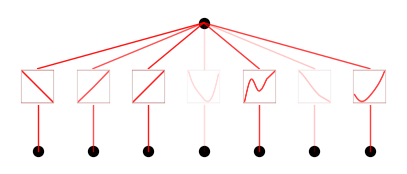
ckan = CoxKAN(width=[2,1], grid=5, seed=42)

_ = ckan.train(
    df_train,
    df_test,
    duration_col='duration',
    event_col='event',
    opt='Adam',
    lr=0.01,
    steps=100)

# evaluate CoxKAN
cindex = ckan.cindex(df_test)
print("\nCoxKAN C-Index: ", cindex)

# plot CoxKAN
fig = ckan.plot()

train loss: 2.77e+00 | val loss: 2.50e+00: 100%|██████████████████| 100/100 [00:06<00:00, 15.48it/s]

CoxKAN C-Index:  0.7553786667818724

Symbolic Fitting:

# auto-symbolic fitting
_ = ckan.auto_symbolic(lib=['x^2', 'sin', 'exp', 'log', 'sqrt', 'tanh'], verbose=False)

# train affine parameters
_ = ckan.train(df_train, df_test, duration_col='duration', event_col='event', opt='LBFGS', steps=10)

display(ckan.symbolic_formula(floating_digit=1)[0][0])

train loss: 2.77e+00 | val loss: 2.50e+00: 100%|████████████████████| 10/10 [00:01<00:00,  8.19it/s]

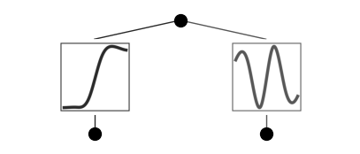
$\displaystyle - 1.0 \sin{\left(6.3 x_{2} + 9.4 \right)} + 1.0 \tanh{\left(4.4 x_{1} \right)}$

We see CoxKAN approximately recovers the true log-partial hazard:

\(\hat{\theta}_{KAN} = \tanh(4.4 x_1) -\sin(6.3 x_2 + 9.4) \approx \tanh(5 x_1) -\sin(2 \pi x_2 + 3 \pi) = \tanh(5 x_1)+ \sin(2 \pi x_2)\)

Real dataset example

from coxkan.datasets import gbsg

# load dataset
df_train, df_test = gbsg.load(split=True)
name, duration_col, event_col, covariates = gbsg.metadata()

# init CoxKAN
ckan = CoxKAN(width=[len(covariates), 1], seed=42)

# pre-process and register data
df_train, df_test = ckan.process_data(df_train, df_test, duration_col, event_col, normalization='standard')

# train CoxKAN
_ = ckan.train(
    df_train,
    df_test,
    duration_col=duration_col,
    event_col=event_col,
    opt='Adam',
    lr=0.01,
    steps=100)

print("\nCoxKAN C-Index: ", ckan.cindex(df_test))

# Auto symbolic fitting
fit_success = ckan.auto_symbolic(verbose=False)
display(ckan.symbolic_formula(floating_digit=2)[0][0])

# Plot coxkan
fig = ckan.plot(beta=20)

Using default train-test split (used in DeepSurv paper).

train loss: 2.60e+00 | val loss: 2.41e+00: 100%|██████████████████| 100/100 [00:01<00:00, 55.04it/s]

CoxKAN C-Index:  0.6798424912829145

$\displaystyle \begin{cases} 0.06 & \text{for}\: meno = 0 \\0.22 & \text{for}\: meno = 1.0 \\\text{NaN} & \text{otherwise} \end{cases} + \begin{cases} 0.23 & \text{for}\: hormon = 0 \\-0.11 & \text{for}\: hormon = 1.0 \\\text{NaN} & \text{otherwise} \end{cases} + \begin{cases} -0.16 & \text{for}\: size = 0 \\0.09 & \text{for}\: size = 1.0 \\0.36 & \text{for}\: size = 2.0 \\\text{NaN} & \text{otherwise} \end{cases} + 0.759 - 1.16 e^{- 0.03 \left(- nodes - 0.58\right)^{2}} - 0.32 e^{- 5.59 \left(0.02 age - 1\right)^{2}}$